Urban Mobility Synthesis | Prabin Bhandari

With Antonios Anastasopoulos and Dieter Pfoser · George Mason University
Best Paper Award · ACM SIGSPATIAL 2024

SIGSPATIAL '24 paper TSAS journal paper arXiv Code & data Model

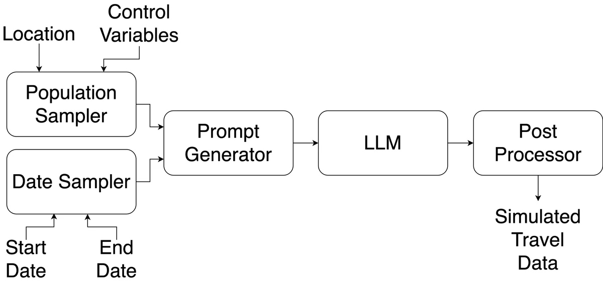
Travel surveys such as the U.S. National Household Travel Survey (NHTS) tell planners where people go over a day, but they are expensive, slow and privacy-sensitive, and few people answer them: the 2017 NHTS had a response rate of 15.6%. We asked whether a large language model can take the participant’s place. Describe a person using census statistics, give a date, and let the model fill in that day’s travel diary. Repeat for thousands of people and you have a synthetic travel survey.

The approach was introduced at ACM SIGSPATIAL 2024, where it received the Best Paper Award, and extended in ACM Transactions on Spatial Algorithms and Systems (TSAS) with newer models, age-balanced fine-tuning and a test of seasonal behavior.

10,000real diaries are enough to fine-tune an open model

43.7%overlap with real daily activity chains, vs 1.4–25.4% for prompted models

5 metrosacross the U.S. evaluated, from San Francisco to Minneapolis

−34%error in age-group travel patterns after age-balanced fine-tuning

Pipeline: population sampler and date sampler feed a prompt generator, then the LLM, then a post-processor that outputs simulated travel data — The pipeline (TSAS Fig. 1). A population sampler draws people from American Community Survey statistics for a metro area, a date sampler picks the survey day, the prompt generator writes a diary prompt, the LLM fills it in, and a post-processor turns the table into a sequence of activities.

From prompt to diary

The prompt reads like the instructions a survey participant receives. The person, place and date (highlighted) change for every sample:

Prompt (abridged)TSAS, Fig. A1

The individual is a 59-year-old female whose racial background is
"White alone". Currently, she is not enrolled in school and is
participating in the labor force. She is employed and working in the
"Business and financial operations occupations" field. […] She lives in
San Francisco, CA. She has been selected for a travel survey and has recorded
her travel logs for 2016-05-05 which is a Thursday. […]

| Place Visited | Arrival Time | Departure Time | Location Type |
|---------------|--------------|----------------|---------------|
| [Place Name]  | [HH:MM AM/PM] | [HH:MM AM/PM] | [Location Type] |

She was reminded of the following:
1. Ensure that "Home" is included in the list if it was part of
   travel activities on the specified date. […]

For the "Location Type," she was instructed to use the corresponding
code from the provided list:
1: Regular home activities (chores, sleep)
3: Work
11: Buy goods (groceries, clothes, appliances, gas)
13: Buy meals (go out for a meal, snack, carry-out)
… 20 codes in total

The table she created is as follows:

Example output (reformatted)TSAS, Table 1

Place visited	Arrival	Departure	Type
Home	00:00 AM	07:30 AM	1
Work	08:00 AM	05:00 PM	3
Home	05:30 PM	11:59 PM	1

Activity chain:  Home → Work → Home
Travel time:     1 h (the gaps between rows)

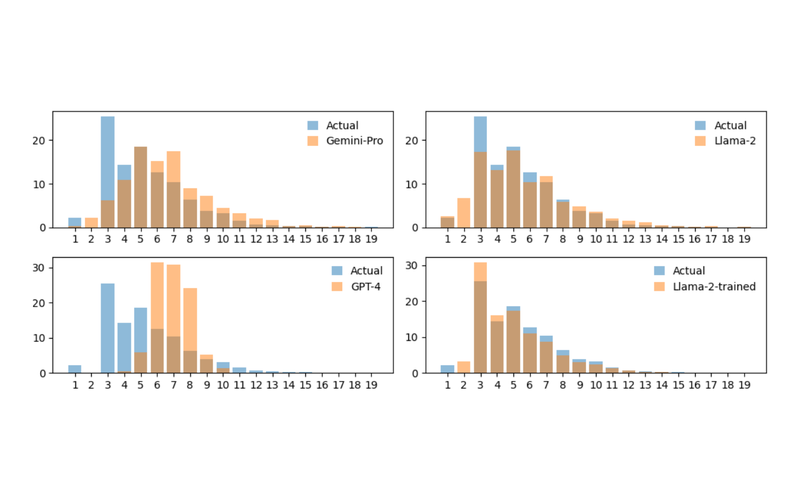
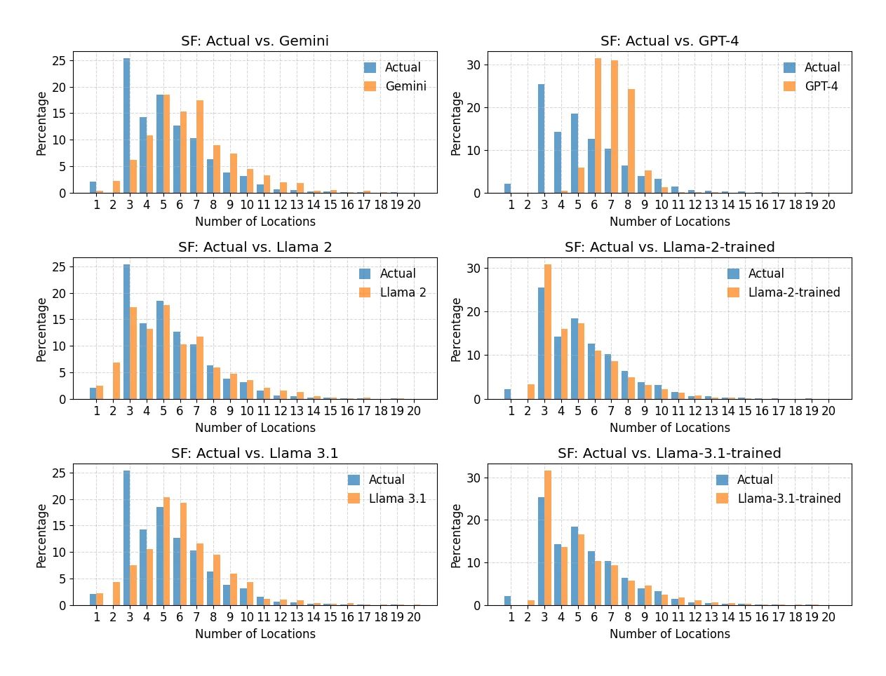
We compare prompted models (Gemini-Pro, GPT-4, Llama-2, Llama-3.1) with Llama-2 and Llama-3.1 fine-tuned with LoRA on 10,000 anonymized NHTS diaries, and evaluate at three levels: daily patterns (places visited, travel time), trips (transitions between activity types) and complete daily activity chains.

Results in San Francisco

Model	Places / day	Travel h / day	Transition error ↓	Chain overlap % ↑
Real survey (NHTS 2017)	5.35	1.74	–	–
Prompted
Gemini-Pro	6.59	2.52	0.063	17.25
GPT-4	6.96	2.52	0.166	1.44
Llama-2	5.55	7.17	0.106	25.42
Llama-3.1	6.05	3.52	0.103	13.96
Fine-tuned on 10,000 diaries
Llama-2-trained	4.97	1.53	0.044	42.54
Llama-3.1-trained	5.29	1.52	0.041	43.74

San Francisco–Oakland–Hayward, from Tables 5–7 of the TSAS paper; closest to the real survey highlighted. Transition error is the Frobenius norm between real and generated first-order transition matrices; chain overlap is the frequency-weighted overlap between real and generated daily activity chains.

Prompted models know roughly what a day looks like but exaggerate it, visiting too many places and, in Llama-2’s case, traveling for hours. After fine-tuning, both open models land close to the real survey on every measure. Generated chains that never appear in the real data are mostly near misses: for the fine-tuned Llama-3.1, 63% of them are a single edit away from a real chain.

Six histograms of places visited per day, real versus each model; the two fine-tuned models match the real distribution most closely — Places visited per day: real survey (blue) vs each model (orange). The fine-tuned models in the bottom row track the real distribution (TSAS Fig. 2).

Other cities

The same models generate surveys for four more metropolitan areas. Weighted overlap of daily activity chains with each city’s real survey:

Metro area	Gemini-Pro	GPT-4	Llama-2	Llama-2-trained	Llama-3.1-trained
Washington–Arlington–Alexandria	18.89	2.7	26.58	40.15	41.56
Los Angeles–Long Beach–Anaheim	17.22	1.51	27.29	43.12	42.62
Dallas–Fort Worth–Arlington	18.4	2.04	28.18	44.42	51.47
Minneapolis–St. Paul–Bloomington	16.99	2.27	24.44	45.84	43.06

Weighted chain overlap in %, higher is better (TSAS Table 8).

Local survey data is not required. A Llama-2 model fine-tuned with all five study metros removed from its training data performs almost the same in San Francisco (4.79 vs 4.97 places per day, 1.60 vs 1.53 hours of travel), so the method can produce surveys for places that have none.

Getting the details right: age and seasons

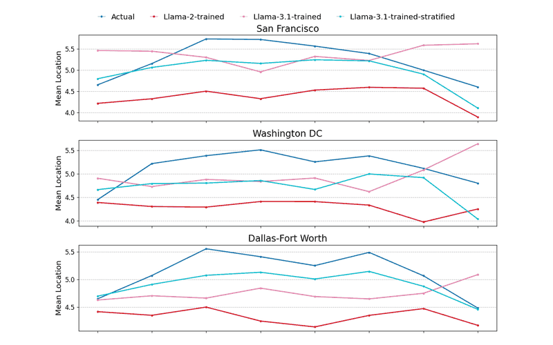
Age. The NHTS over-represents older adults compared with the census. Fine-tuning Llama-3.1 on a sample balanced by age and sex recovers the real “inverted-U” profile, where people in mid-life visit the most places, and cuts the age-profile error by 34% on average with almost no change in the city-level results.

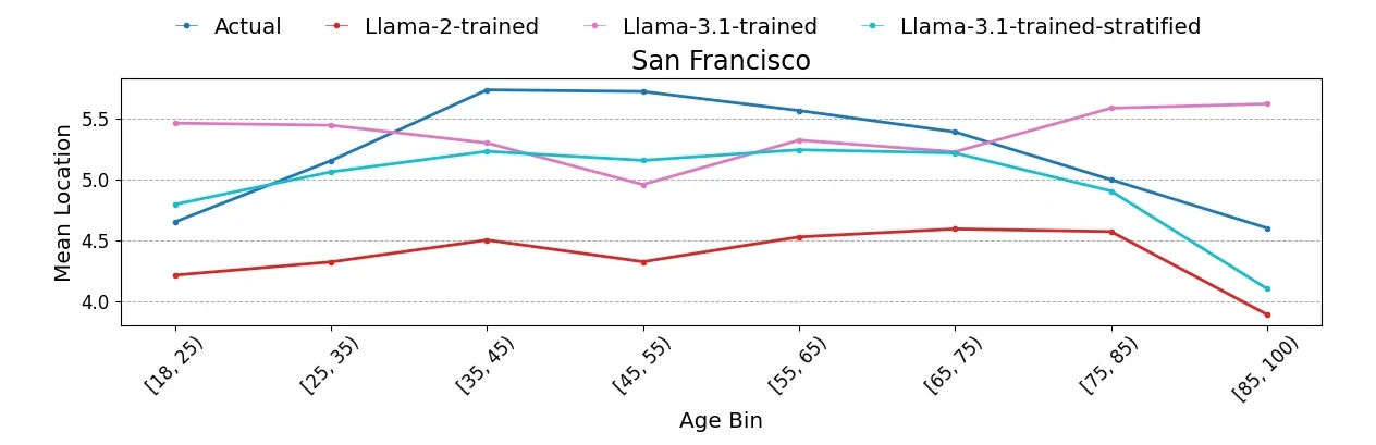
Line chart of mean places visited by age group in San Francisco; the stratified model follows the real inverted-U curve more closely than the other fine-tuned models — San Francisco: places visited per day by age group. The age-balanced model (teal) follows the real curve (blue); San Francisco panel of TSAS Fig. 10.

City	Llama-2-trained	Llama-3.1-trained	Llama-3.1, age-balanced
San Francisco	0.9189	0.6112	0.3527
Washington DC	0.9123	0.5651	0.5129
Dallas–Fort Worth	0.8704	0.5873	0.2635
Los Angeles	0.9252	0.6226	0.4321
Minneapolis	0.6573	0.5856	0.4148
Mean	0.8568	0.5944	0.3952

RMSE of mean places visited per age group against the real survey, lower is better (TSAS Table 10). The full-precision Llama-3.1 also beats the 8-bit Llama-2 by a wide margin here, a gap that city-level averages hide.

Seasons. The model is never told about the weather, yet its surveys rise and fall with temperature the way real ones do. The correlation between monthly temperature and monthly activity is 0.85 for generated data in New York (real: 0.83), 0.45 in Los Angeles (real: 0.22) and 0.57 in Dallas–Fort Worth (real: 0.37). In none of the six cities tested does the model invert the relationship.

Compared with a rule-based simulation

Against Patterns of Life, a conventional agent-based simulation, the LLM-generated surveys match the spread of places visited more closely, including the busy days in the tail, and reproduce more of the rare activity chains that the rule-based model never produces.

From surveys to simulation

Each synthetic diary here is a single independent day. UrbanLLMind turns the idea into a running city: persistent agents that plan, remember and react over a week, evaluated with the same three-level framework.

Publications

ACM TSAS
Behaviorally Realistic Urban Mobility Synthesis via Fine-Tuned Large Language Models

Prabin Bhandari, Antonios Anastasopoulos, and Dieter Pfoser

ACM Trans. Spatial Algorithms Syst., Jul 2026

Abs DOI Bib HTML PDF

In urban science, understanding mobility patterns is essential for improving the quality of life and designing livable, efficient, and sustainable cities. However, collecting such data through user tracking or travel surveys poses challenges due to privacy concerns, non-compliance, and high cost. This work proposes an AI-based approach for synthesizing travel surveys by prompting large language models (LLMs), leveraging their background knowledge and text generation capabilities. We evaluate the effectiveness of this method across five major U.S. metropolitan areas by comparing LLM-generated results with existing survey data at three different levels of granularity: (i) pattern level, which compares aggregated metrics like average locations visited and travel time, (ii) trip level, which compares trips as whole units using transition probabilities, and (iii) activity chain level, which examines the sequence of visited places. Our results indicate that fine-tuning an open-weight Llama-3.1 model on a balanced dataset helps approximate age-specific mobility profiles, producing outputs that closely resemble demographic realities. Furthermore, we observe that the model captures implicit seasonal variations in mobility patterns, reproducing fluctuations associated with temperature despite not being given explicit climate inputs. These findings suggest that LLMs, when fine-tuned on as few as 10,000 survey records, can generate synthetic travel data that approximates behavioral realism in major urban contexts. While further validation is needed for non-metropolitan areas and granular transportation metrics, this approach offers a scalable, low-cost, and privacy-preserving complement for urban mobility analysis.
@article{10.1145/3816246, author = {Bhandari, Prabin and Anastasopoulos, Antonios and Pfoser, Dieter}, title = {Behaviorally Realistic Urban Mobility Synthesis via Fine-Tuned Large Language Models}, year = {2026}, issue_date = {December 2026}, publisher = {Association for Computing Machinery}, address = {New York, NY, USA}, volume = {12}, number = {4}, issn = {2374-0353}, url = {https://doi.org/10.1145/3816246}, doi = {10.1145/3816246}, journal = {ACM Trans. Spatial Algorithms Syst.}, month = jul, articleno = {19}, numpages = {33}, keywords = {Large language models, travel data, travel survey, travel survey data simulation, urban mobility}, }
SIGSPATIAL
Urban Mobility Assessment Using LLMs

Prabin Bhandari, Antonios Anastasopoulos, and Dieter Pfoser

In Proceedings of the 32nd ACM International Conference on Advances in Geographic Information Systems, Atlanta, GA, USA, Nov 2024

Best Paper Award Abs DOI Bib HTML PDF Code

Best Paper Award at ACM SIGSPATIAL 2024, Atlanta, GA.

In urban science, understanding mobility patterns and analyzing how people move around cities helps improve the overall quality of life and supports the development of more livable, efficient, and sustainable urban areas. A challenging aspect of this work is the collection of mobility data through user tracking or travel surveys, given the associated privacy concerns, noncompliance, and high cost. This work proposes an innovative AI-based approach for synthesizing travel surveys by prompting large language models (LLMs), aiming to leverage their vast amount of relevant background knowledge and text generation capabilities. Our study evaluates the effectiveness of this approach across various U.S. metropolitan areas by comparing the results against existing survey data at different granularity levels. These levels include (i) pattern level, which compares aggregated metrics such as the average number of locations traveled and travel time, (ii) trip level, which focuses on comparing trips as whole units using transition probabilities, and (iii) activity chain level, which examines the sequence of locations visited by individuals. Our work covers several proprietary and open-source LLMs, revealing that open-source base models like Llama-2, when fine-tuned on even a limited amount of actual data, can generate synthetic data that closely mimics the actual travel survey data and, as such, provides an argument for using such data in mobility studies.
@inproceedings{10.1145/3678717.3691221, author = {Bhandari, Prabin and Anastasopoulos, Antonios and Pfoser, Dieter}, title = {Urban Mobility Assessment Using LLMs}, year = {2024}, isbn = {9798400711077}, publisher = {Association for Computing Machinery}, address = {New York, NY, USA}, url = {https://doi.org/10.1145/3678717.3691221}, doi = {10.1145/3678717.3691221}, booktitle = {Proceedings of the 32nd ACM International Conference on Advances in Geographic Information Systems}, pages = {67–79}, numpages = {13}, keywords = {Large Language Models, Travel Data, Travel Survey, Travel Survey Data Simulation}, location = {Atlanta, GA, USA}, series = {SIGSPATIAL '24}, month = nov, }